The Damped Unforced Pendulum Problem
Applying physics-informed neural networks to ODEs
Introduction: Understanding the Damped Pendulum Problem

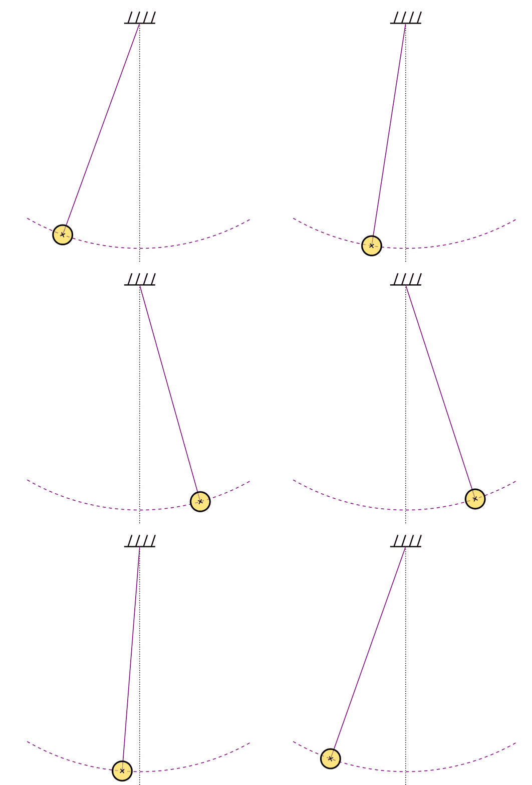
The pendulum problem is a fundamental problem in classical mechanics and as such is often one of the topics taught to first year physics students in college. The earliest well-known use of pendulums in modern history dates back to 1656 when the Dutch scientist Christiaan Huygens used a pendulum as a time-keeping device.
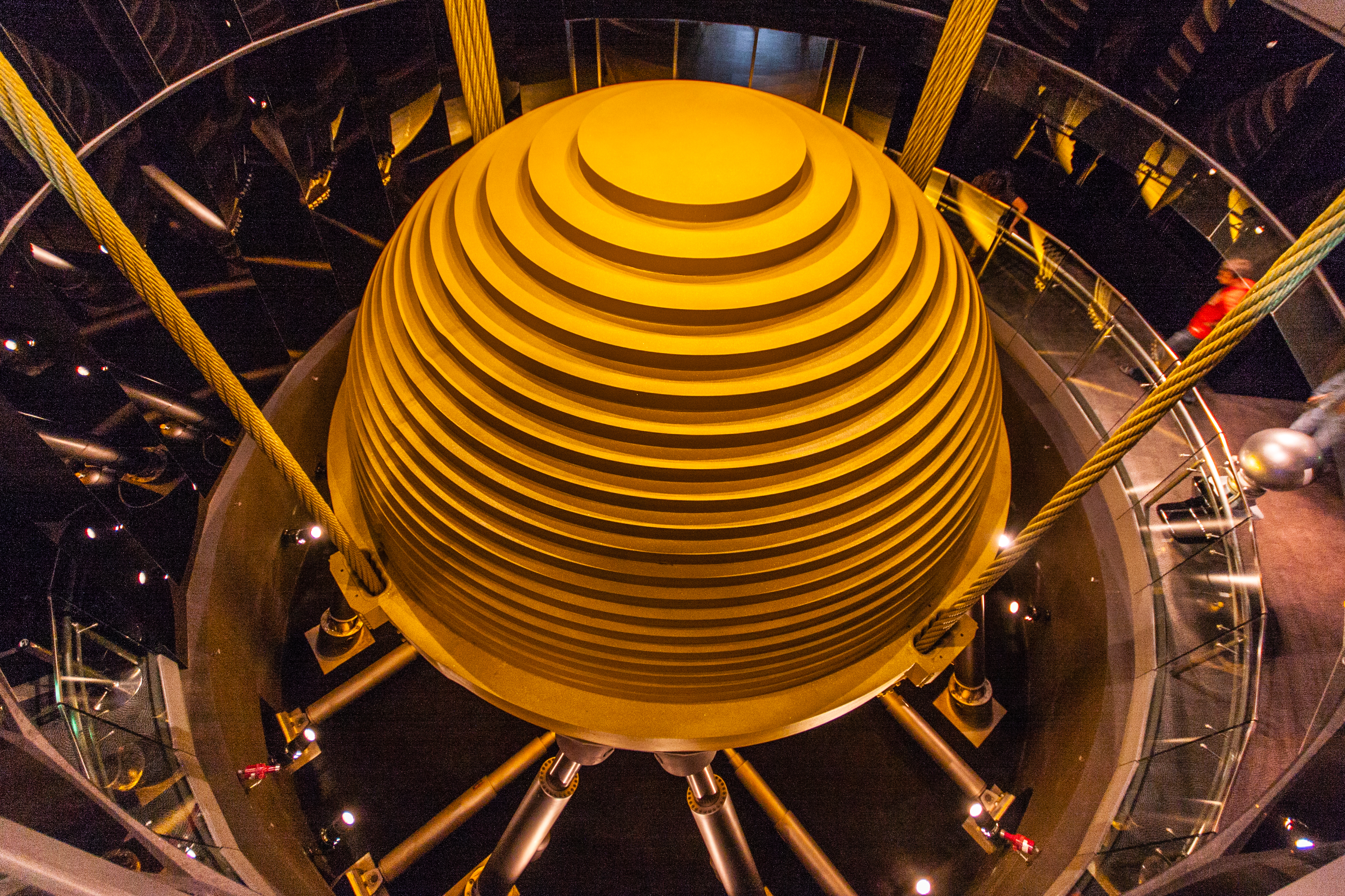
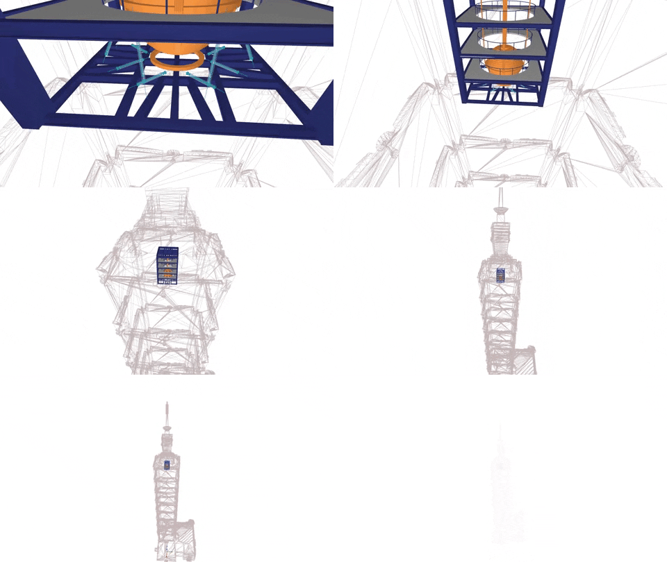
The utility of the pendulum, however, extends far beyond its historical significance. Indeed, the pendulum problem is quite important in modern science and engineering. In fact, the underlying principles driving the behaviour of the pendulum are foundational in understanding the topics of harmonic motion and vibration control. These topics are particularly important in fields such as seismology and structural engineering. For example, pendulums are key components in the design of classical seismographs where they are used to measure and record the strength and duration of earth tremors and earthquakes. Such an application is pivotal in the field of seismic monitoring as it aids in the prediction of seismic events, thereby significantly improving public safety. Furthermore, structural engineers often employ pendulum principles in the design of systems and elements that would improve a building’s seismic resilience. More specifically, tuned mass dampers are used to mitigate the vibrations in structures caused by winds and earthquakes.
The development of pendulum motion analysis within a dynamical systems framework has been a significant leap in the understanding of the pendulum problem in realistic
However, as the applications of pendulum principles grow increasingly complex, the corresponding dynamical systems modeling the desired behaviors become harder and harder to solve and analyze. Historically, this gave rise to the field of numerical analysis, which focused on developing various numerical schemes that are provably reliable in order to solve problems with no analytic
As we stand on the brink of a new frontier in dynamical systems analysis, it is clear that our journey with the pendulum, from a simple timekeeping device to a complex model in engineering and physics has been nothing short of remarkable. The pendulum’s story teaches us the value of revisiting basic concepts with a fresh perspective, continually pushing the boundaries of our understanding and capabilities. In this era of rapid technological advancement, our quest to model and predict complex dynamical systems is more relevant than ever. It paves the way for innovative solutions that are not just faster and more precise, but also more accessible to a wider range of applications. This evolution in approach, subtly hinted at, but not yet fully explored, promises to revolutionize how we perceive and interact with the dynamic world around us. It faithfully embodies the very spirit of continuous discovery and improvement that drives the scientific effort.
Data Foundations: Pendulum Dynamics and Parameters
This project is designed within the analysis framework of dynamical systems theory which attempts to model real-world time dependent systems referred to as ‘dynamical systems’. In particular the specifc model for the pendulum problem was chosen with a fine balance between realistic behavior and model complexity in mind. The two sub-sections below introduce the theoretical framework for modeling pendulum motion and explain the data generation process used to collect the data needed for training the Vanilla neural network model introduced in the next section.
The Theoretical Framework
The traditional 1D damped unforced pedulum problem is modeled by the second order homogenous constant coefficient non-linear oridinary differential equation (ODE):
\[\ddot{\theta}(t)+b \dot{\theta}(t)+\frac{g}{L} \sin (\theta(t))=0\]where
- \(\ddot{\theta}(t)\) is the second derivative of \(\theta(t)\) with respect to time, representing the angular acceleration of the pendulum (\(rad/s^2\)).
- \(\dot{\theta}(t)\) is the first derivative of \(\theta(t)\) with respect to time, representing the angular velocity of the pendulum (\(rad/s\)).
- \(b\) is the damping coefficient, representing the effect of air resistance or other damping forces.
- \(g\) is the acceleration due to gravity.
- \(L\) is the length of the pendulum.
Since the equation above is non-linear in nature, it does not have a closed-form solution. This, in turn, necessitates the use of numerical methods such as the those from the Runge-Kutta, Adams-Bashford and Adams-Moulton families of methods. It is important to note that throughout this article the notation,
\[\omega(t) = \dot{\theta}(t)\]will be used for convenience and in accordance with the classical mechanics nomenclature.
Data Generation
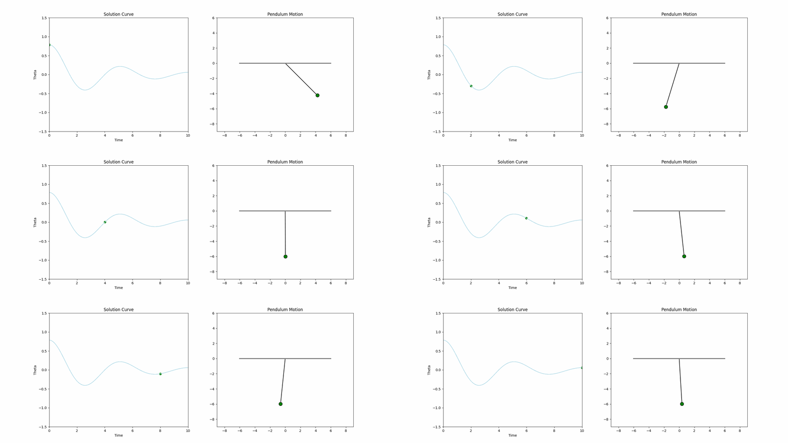
An initial value problem (IVP) with parameters $b=0.5$, $g=9.81$ and $L=6$, and initial conditions $\theta(0)=\frac{\pi}{4}$ and $\omega(0)=0$ is used to generate data for the pendulum problem. The particular form of the IVP is written as
\[\begin{aligned} \ddot{\theta}(t)+0.5 \dot{\theta}(t)+\frac{9.81}{6} \sin (\theta(t)) & =0, \\ \theta(0) & =\frac{\pi}{4}, \\ \dot{\theta}(0) & =0 . \end{aligned}\]This form of the IVP, however, is not the standard form accepted by numerical solvers, which require a first order form. To convert the IVP to a first order form it is necessary to express it as a system of two first order ODEs with a corresponding vector of initial conditions. This can be done, by letting
\[\begin{aligned} \dot{\theta}(t) & =\omega(t) \\ \dot{\omega}(t) & =-0.5 \omega(t)-\frac{9.81}{6} \sin (\theta(t)) \end{aligned}\]which then results in the linear system of first order ODEs with an initial value vector
\[\left[\begin{array}{c} \dot{\theta}(t) \\ \dot{\omega}(t) \end{array}\right]=\left[\begin{array}{c} \omega(t) \\ -0.5 \omega(t)-\frac{9.81}{6} \sin (\theta(t)) \end{array}\right], \quad\left[\begin{array}{c} \theta(0) \\ \omega(0) \end{array}\right]=\left[\begin{array}{l} \frac{\pi}{4} \\ 0 \end{array}\right]\]The specific numerical solver used to solve the IVP above and generate the training data is the solve_ivp function from the Python scipy library. The underlying numerical method employed is the Runge-Kutta order 5 method, which is appropriate in this situation since the underlying ODE is not stiff. Below is the short code used to generate the training data for the Vanilla Neural Network.
import numpy as np
from scipy.integrate import solve_ivp

# Constants
b = 0.5 # damping coefficient
g = 9.81 # acceleration due to gravity
L = 6 # length of the pendulum
y0 = [np.pi/4, 0] # Initial conditions

# Differential Equation
def damped_pendulum(t, y):
    theta, omega = y
    dtheta_dt = omega
    domega_dt = -b * omega - (g / L) * np.sin(theta)
    return [dtheta_dt, domega_dt]

# Generate and solve ODE
def generate_ode_solution(t_span, y0, t_eval):
    return solve_ivp(damped_pendulum, t_span, y0, t_eval=t_eval)
Finally, note that due to the nature of the ODE problem, there is no need for specific training, validation and test datasets. Both of the models presented in the next section will learn the IVP solution, namely \(\theta(t)\) and \(\omega(t)\), on the pre-specified domain
Modeling Pendulum Motion: Neural Network Approaches
This section presents two different Neural Network models that are trained to predict the values of the IVP presented in Data Generation. The first model is a Vanilla Neural Network that uses the true \(\theta\) and \(\omega\) data obtained via the numerical solver solve_ivp and outputs \(\widehat{\theta}\) and \(\widehat{\omega}\). The reason for choosing the VNN model is for its function approximation properties and to have it serve as a control model for the more complicated Physics-Informed model.
The Vanilla Neural Network
A simple neural network model, referred to as a “Vanilla Neural Network”, was selected as the control model to compare with the physics-informed neural network introduced in the next section. The VNN model consists of a simple feed-forward neural network with 1 input node for the \(t\)-values and 3 hidden layers with 32 units each, activated with a hyperbolic tangent function \(\tanh\). There are two output nodes, one for \(\widehat{\theta}\) and another for \(\widehat{\omega}\). The Loss function is custom-defined to use the sum of the \(\operatorname{MSE}\) (mean squared error) for \(\widehat{\theta}\) and \(\widehat{\omega}\) and is given by
\[\begin{align*} \operatorname{Loss}_{\mathrm{TOTAL}} &= \operatorname{MSE}(\widehat{\theta}, \theta) + \operatorname{MSE}(\widehat{\omega}, \omega) \\ &= \frac{1}{n} \sum^{n}_{i=1}(\widehat{\theta}_i - \theta_i)^2 + \frac{1}{n} \sum^{n}_{i=1}(\widehat{\omega}_i - \omega_i)^2 \\ &= \frac{1}{n} \sum^{n}_{i=1}(\widehat{\theta}_i - \theta_i)^2 + (\widehat{\omega}_i - \omega_i)^2 \end{align*}\]Outside of the custom defined mean-squared loss function, which is otherwise indifferent to the standard \(\operatorname{MSE}\) loss function in keras, the neural network architecture is identical to that of the standard FFNNs. Below is a diagram of the structure that was described above.
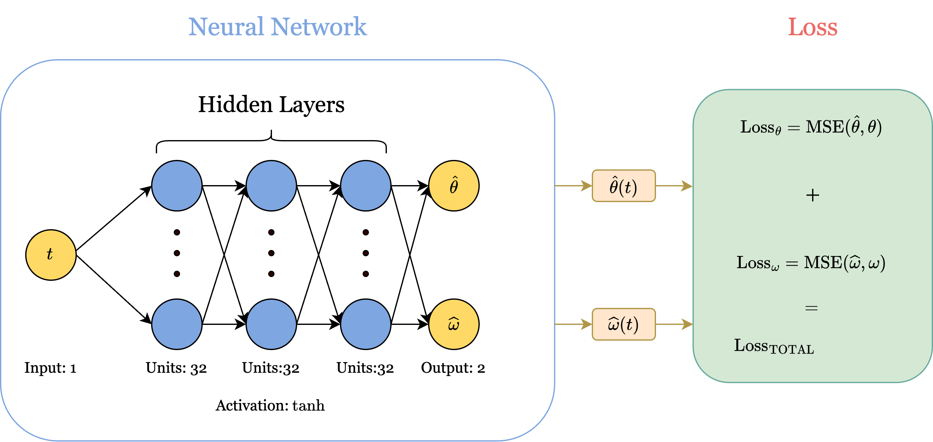
The particular implementation in Python of the model can be seen below. For the full details, please refer to the project code link in the Appendix.
import tensorflow as tf

# Neural Network Model
class DampedPendulumModel(tf.keras.Model):
    def __init__(self):
        super().__init__()
        self.layers_list = [tf.keras.layers.Dense(units=32, activation='tanh') for _ in range(3)]
        self.output_layer = tf.keras.layers.Dense(units=2)

    def call(self, inputs):
        x = inputs
        for layer in self.layers_list:
            x = layer(x)
        return self.output_layer(x)

# Vanilla Loss Function
def compute_vanilla_loss(predictions, actual_theta, actual_omega):
    return tf.reduce_mean(tf.square(predictions[:, 0] - actual_theta)

                          + tf.square(predictions[:, 1] - actual_omega))

# Vanilla NN Training Function
def train_vanilla(model, optimizer, t_data, theta_data, omega_data, epochs):
    train_loss_record = []
    plot_filenames = []
    for epoch in range(epochs):
        with tf.GradientTape() as tape:
            predictions = model(tf.constant(t_data.reshape(-1, 1), dtype=tf.float32))
            loss = compute_vanilla_loss(predictions, theta_data, omega_data)
        grads = tape.gradient(loss, model.trainable_variables)
        optimizer.apply_gradients(zip(grads, model.trainable_variables))
        train_loss_record.append(loss.numpy())
    return train_loss_record, plot_filenames
Note that the GradientTape method in tensorflow is used to record operations that would later be differentiated with the gradient method. This is TensorFlow’s approach to allowing the implementation of custom loss functions by users in Python.
The Physics-Informed Neural Network
Physics-Informed Neural Networks (PINNs), despite their novelty, are well known for their useful properties in the study and solution of differential equations.
The particular PINN that was chosen to learn and predict the behavior of the pendulum IVP, consists of a feed-forward neural network with the same specifications as the one presented in the previous sub-section, and a custom-designed physics-informed loss function which guides its training. The loss function consists of two parts. The first part is the loss contributed from the differential equation which is given as
\[\operatorname{Loss}_{\mathrm{GE}}=\operatorname{MSE}\left(\frac{d \hat{\theta}}{d t}-\widehat{\omega}, 0\right)+\operatorname{MSE}\left(\frac{d \widehat{\omega}}{d t}+b \cdot \widehat{\omega}+\left(\frac{g}{L}\right) \cdot \sin (\hat{\theta}), 0\right)\]where \(\frac{d \hat{\theta}}{d t}\) and \(\frac{d \widehat{\omega}}{d t}\) are the gradients of the predicted \(\theta\) and \(\omega\) and are obtained via automatic differentiation. The second part of the loss function measures the loss contributed from the initial conditions of the IVP, namely \(\theta(0)\) and \(\omega\), and is given as
\[\operatorname{Loss}_{\mathrm{IC}}=\operatorname{MSE}\left(\hat{\theta}_0, \theta_0\right)+\operatorname{MSE}\left(\widehat{\omega}_0, \omega_0\right)\]Then, the total loss is then the sum of the two parts and is given as
\[\operatorname{Loss}_{\mathrm{TOTAL}}=\operatorname{Loss}_{\mathrm{GE}}+\operatorname{Loss}_{\mathrm{IC}}\]Below is a diagram of the architecture of the PINN.
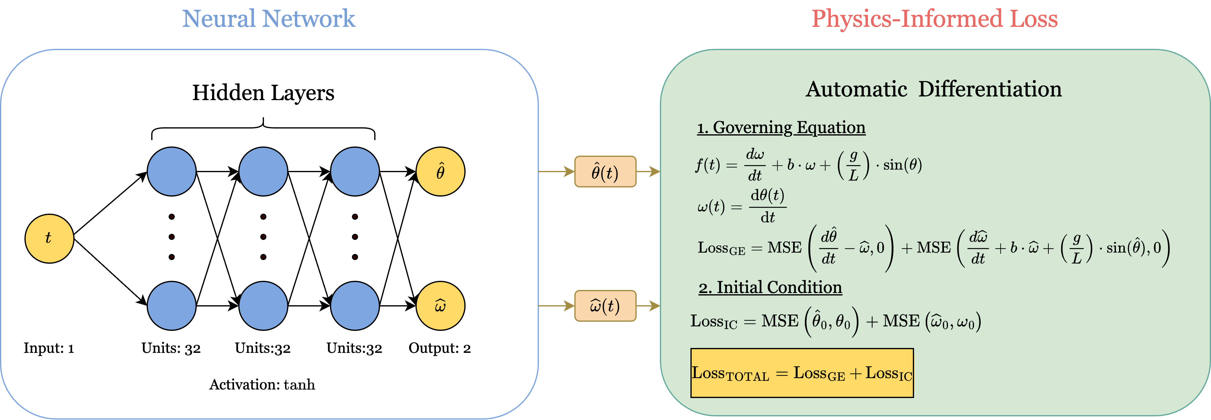
Here is a specific Python implementation of this architecture with tensorflow. Please refer to the Appendix for a link to the entire code.
import tensorflow as tf

# Neural Network Model
class DampedPendulumModel(tf.keras.Model):
    def __init__(self):
        super().__init__()
        self.layers_list = [tf.keras.layers.Dense(units=32, activation='tanh') for _ in range(3)]
        self.output_layer = tf.keras.layers.Dense(units=2)

    def call(self, inputs):
        x = inputs
        for layer in self.layers_list:
            x = layer(x)
        return self.output_layer(x)

# Physics-Informed Loss Function
def compute_loss(model, t_data, y0):
    with tf.GradientTape(persistent=True) as tape:
        tape.watch(t_data)
        predictions = model(t_data)
        theta, omega = predictions[:, 0:1], predictions[:, 1:2]

    # Compute gradients outside the context of the tape
    dtheta_dt = tape.gradient(theta, t_data, unconnected_gradients=tf.UnconnectedGradients.ZERO)
    domega_dt = tape.gradient(omega, t_data, unconnected_gradients=tf.UnconnectedGradients.ZERO)
    del tape  # Delete the persistent tape after gradients are computed

    # Damped pendulum equation
    damped_eq = domega_dt + b * omega + (g / L) * tf.sin(theta)

    # Loss for ODE and initial conditions
    ode_loss = tf.reduce_mean(tf.square(dtheta_dt - omega) + tf.square(damped_eq))
    ic_loss = tf.reduce_mean(tf.square(predictions[0] - y0))
    return ode_loss + ic_loss

# Training Function
def train(model, optimizer, t_data, y0, epochs, t_eval):
    loss_history = []
    for epoch in range(epochs):
        with tf.GradientTape() as tape:
            loss = compute_loss(model, t_data, y0)
        grads = tape.gradient(loss, model.trainable_variables)
        optimizer.apply_gradients(zip(grads, model.trainable_variables))
        loss_history.append(loss.numpy())
    return loss_history
Note that, just like it was for the VNN, the physics informed loss function is incorporated into the model within the train function, where the GradientTape method is used for the loss function’s integration within the TensorFlow back-propagation framework.
Results: Model Outcomes and Insights
This section covers the results of the two models and concludes with a comparison. The first objective is to train the VNN model on \(\theta\) and \(\omega\) data from the time interval \([0,10]\) and demonstrate its ability to accurately approximate the true solutions \(\theta(t)\) and \(\omega(t)\) on that interval. Note that since Neural Networks are by nature universal approximators, training the VNN on the data from the interval \([0,10]\) will allow it to learn the behavior of the dynamical system entirely.
VNN
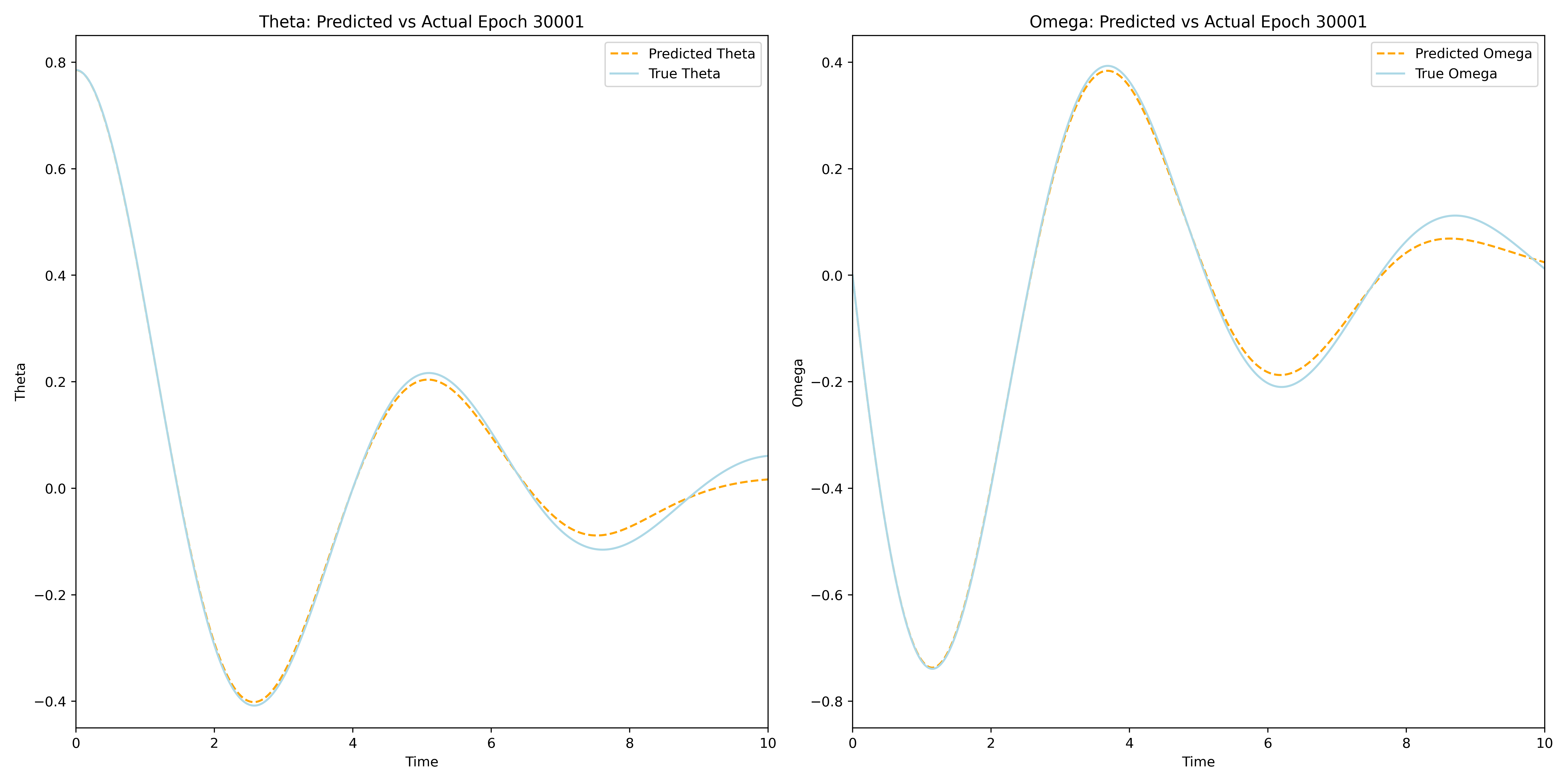
The Vanilla Neural Network model was trained for 30001 epochs on 250 equispaced IVP solution points
The final training epoch resulted in a model that closely approximates the true solution of the IVP on the interval \([0,10]\).
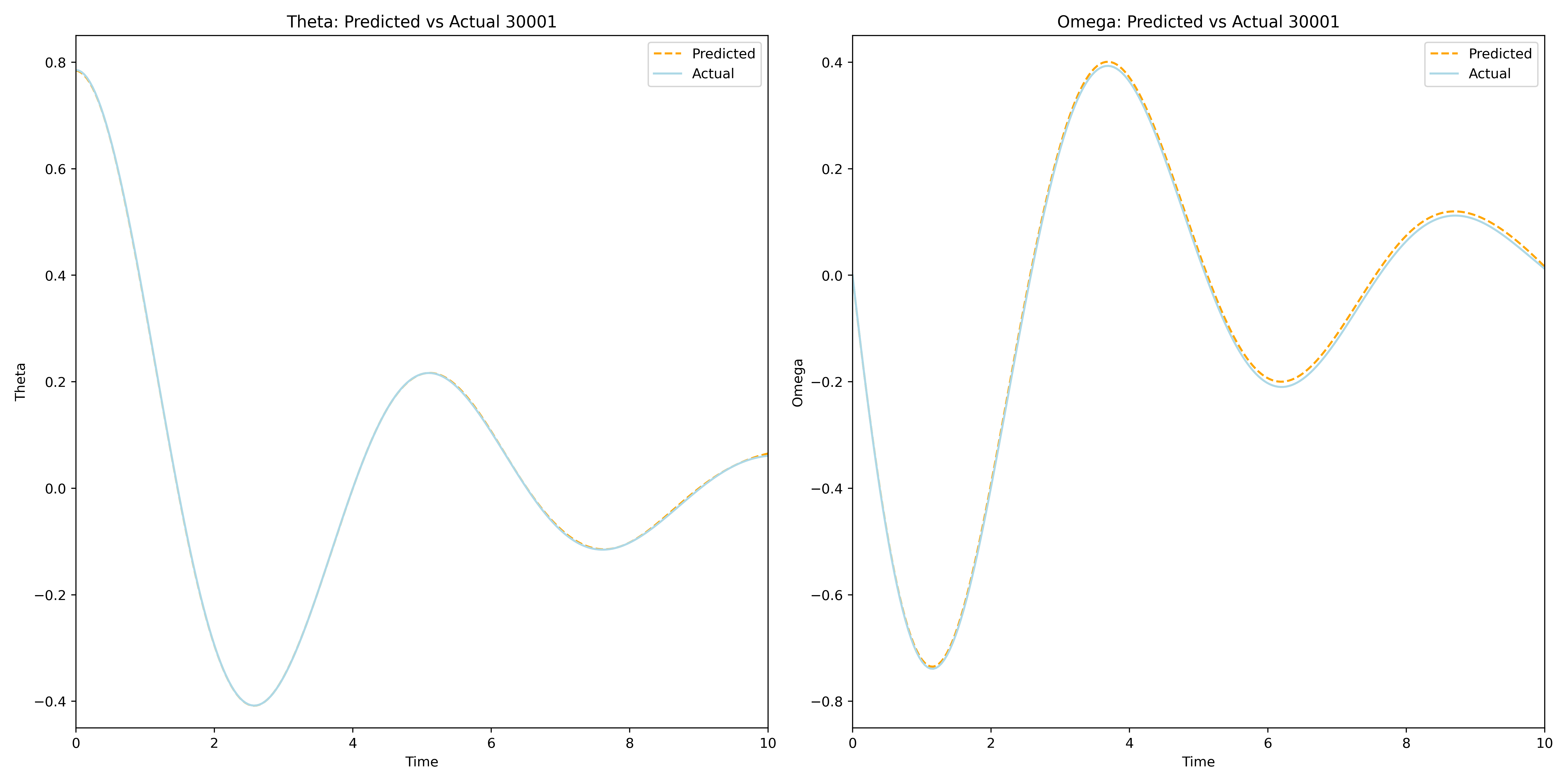
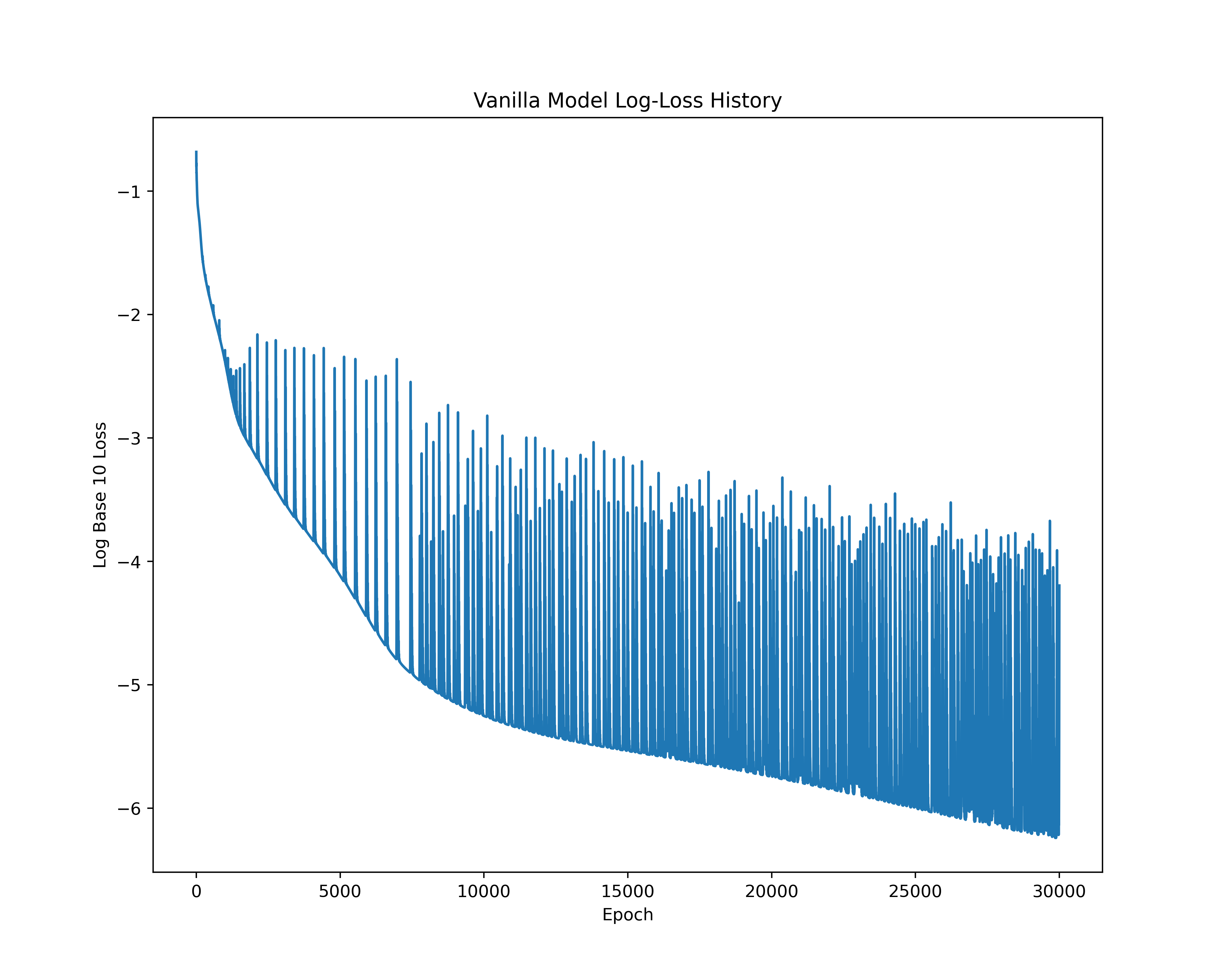
The associated training loss throughout the epochs can be seen in the following log base 10 loss plot.
PINN
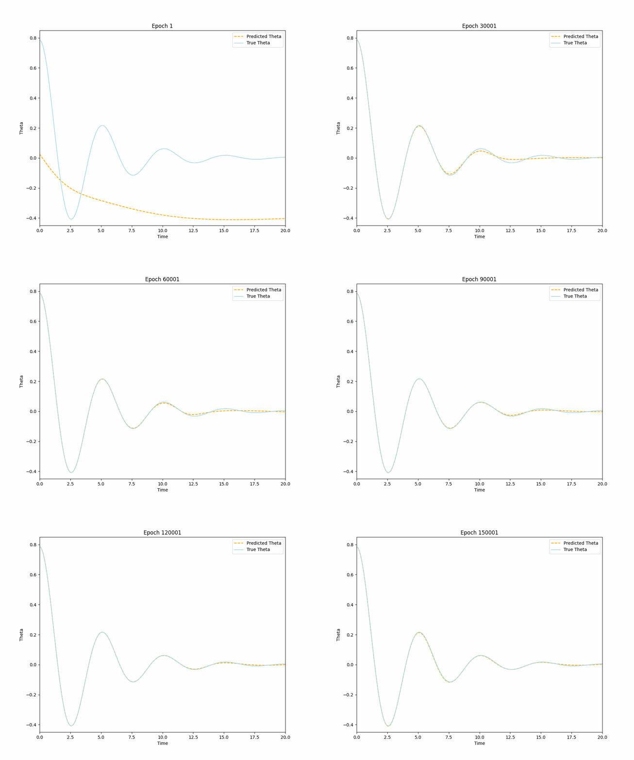
The Physics-Informed Neural Network model was trained for 30001 epochs on 500 points from the interval \([0,20]\). Below is a dynamic visalization of the training process that demonstrates neural networks’ ability to accurately approximate \(\theta(t)\) and \(\omega(t)\) in sufficiently many epochs.
The final training epoch resulted in a model that produces a good approximation of the actual solution, which, however, is not sufficiently good for engineering purposes. For a better approximation of the quality of the VNN approximation more training epochs are needed.
The associated training loss throughout the epochs can be seen in the following log base 10 loss plot.
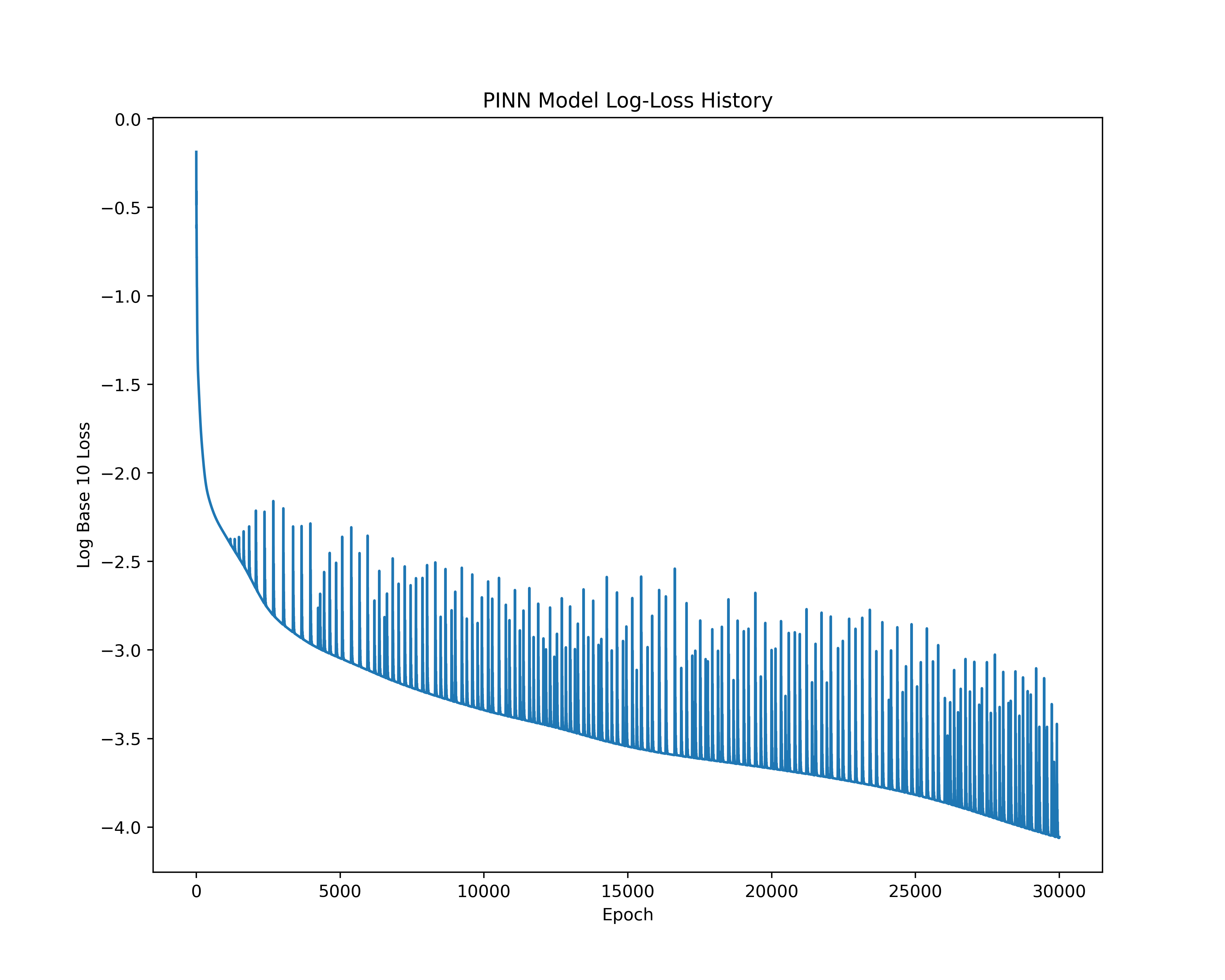
As we can see from the Log 10 plot of the loss throughout the epochs for the PINN model, there is less overfitting as evidenced by the lower jumps in loss at higher epochs. This suggests that the PINN model is a more stable approach for solving the IVP. The reliance on a physics-informed loss function helps mitigate the overfitting issues arising from the underlying structure of ANNs.
Comparison of Results
The VNN and PINN models are two very different approaches to solving the the pendulum IVP. While the Vanilla Neural Network model takes a traditional data-dependent deep learning approach, the Physics-Informed Neural Network uses an entirely novel approach that combines some of the best aspects of the worlds of numerical solvers and deep learning. The non-reliance on training data of the PINN allows it to focus on more accurately learning the underlying dynamics of the problem through its physics-informed loss function. This results in a model that not only requires no-data to train, but also has the ability to almost instantenously predict on the entire interval of training without the need for interpolation. To demonstrate this visually the VNN and PINN models were used to predict the IVP solution on the interval \([0,20]\).
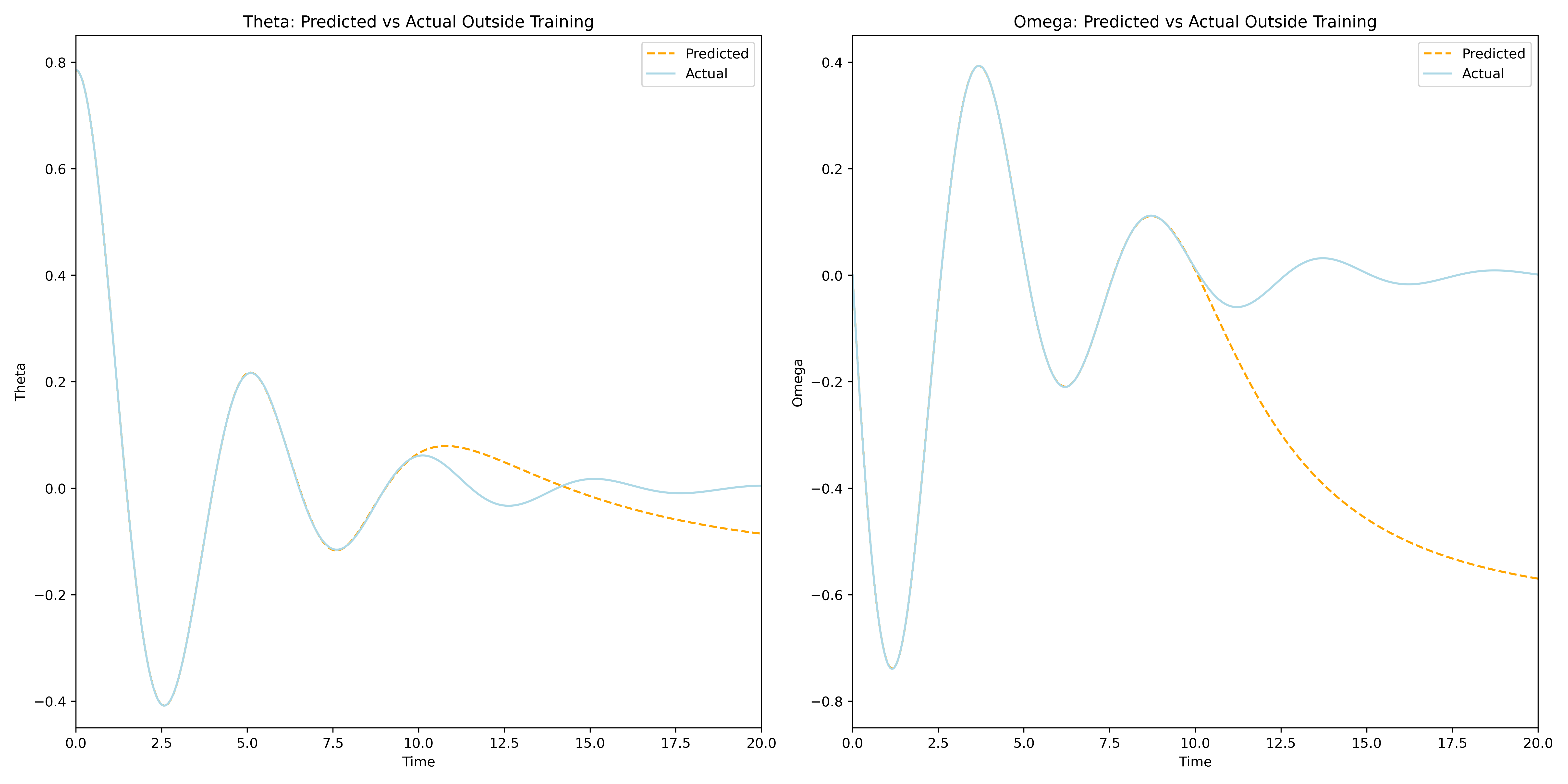
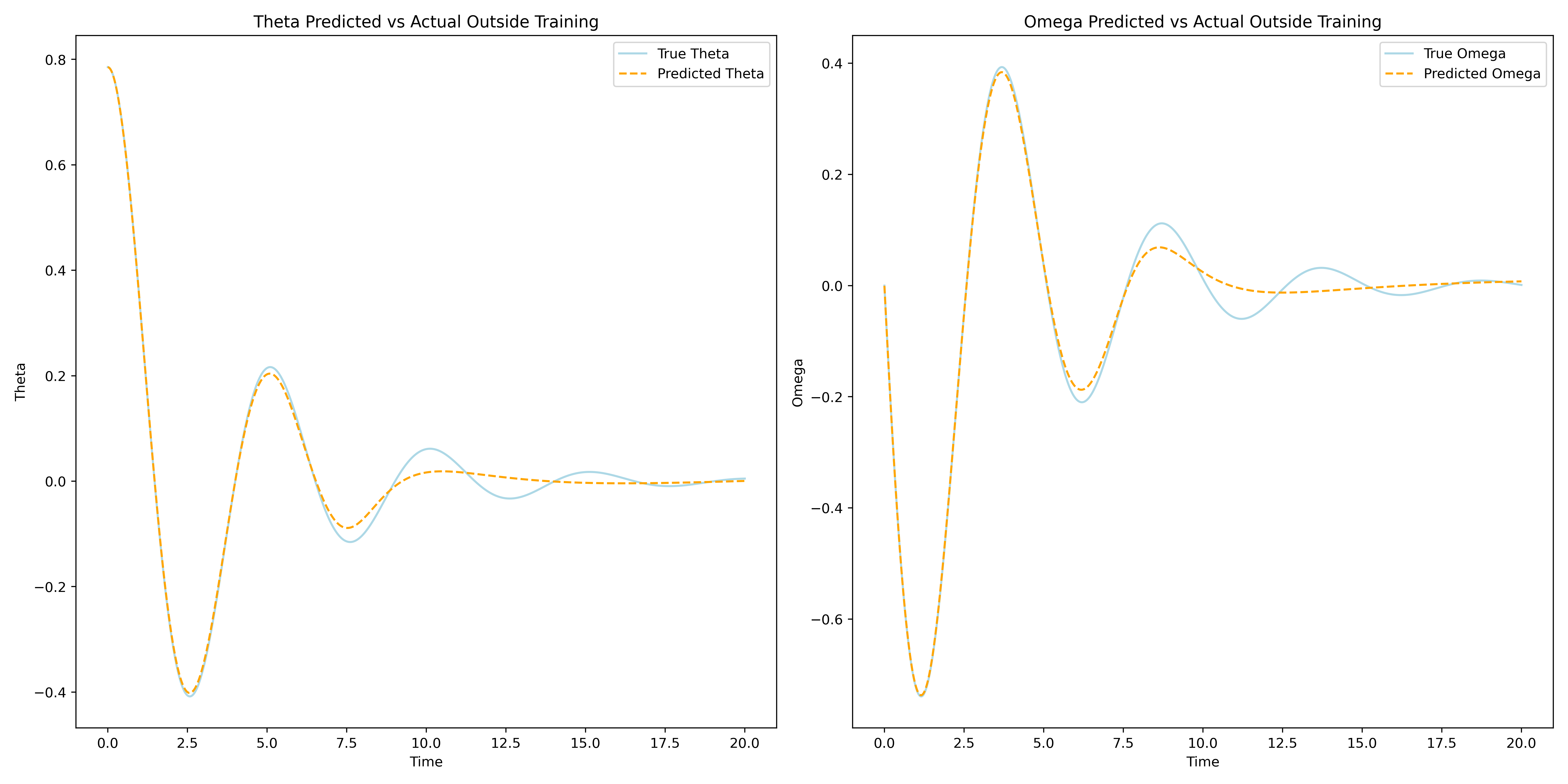
As can be seen from the plots above the Vanilla Neural Network accurately approximates the true solution on its interval of training, but it fails to predict the solution outside of the interval \([0,10]\). This, of course, is to be expected and is an excellent example of typical Neural Networks reliance on training data for making predictions. This over-reliance on data could often mislead or downright prevent engineers and researchers from gaining valuable insights about the problem, especially if the training data is tainted for some reason. The Physics-Informed Neural Network on the other hand demonstrates its ability to learn the IVP solution outside the original interval of interest, without the need to use any training data. This opens the door for a lot of applications of PINNs for solving differential equations that were previously thought unachievable by Neural Networks. With sufficient training one can use a PINN to solve complex differential equations almost instantaneously and to a great degree of accuracy. Below is a dynamic visualization of the training process of a PINN over 150001 epochs on the pendulum IVP.
Neural Networks as Interpolators
An interesting aspect of both the PINN and VNN models, which is also shared by all ANNs
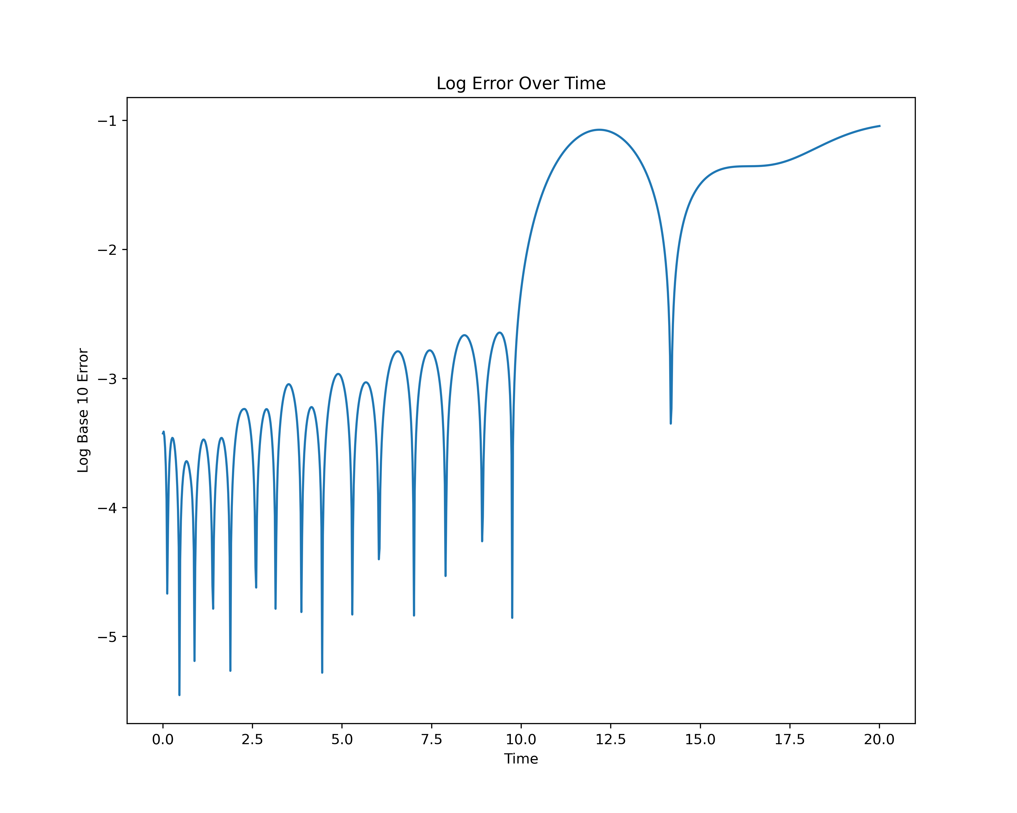
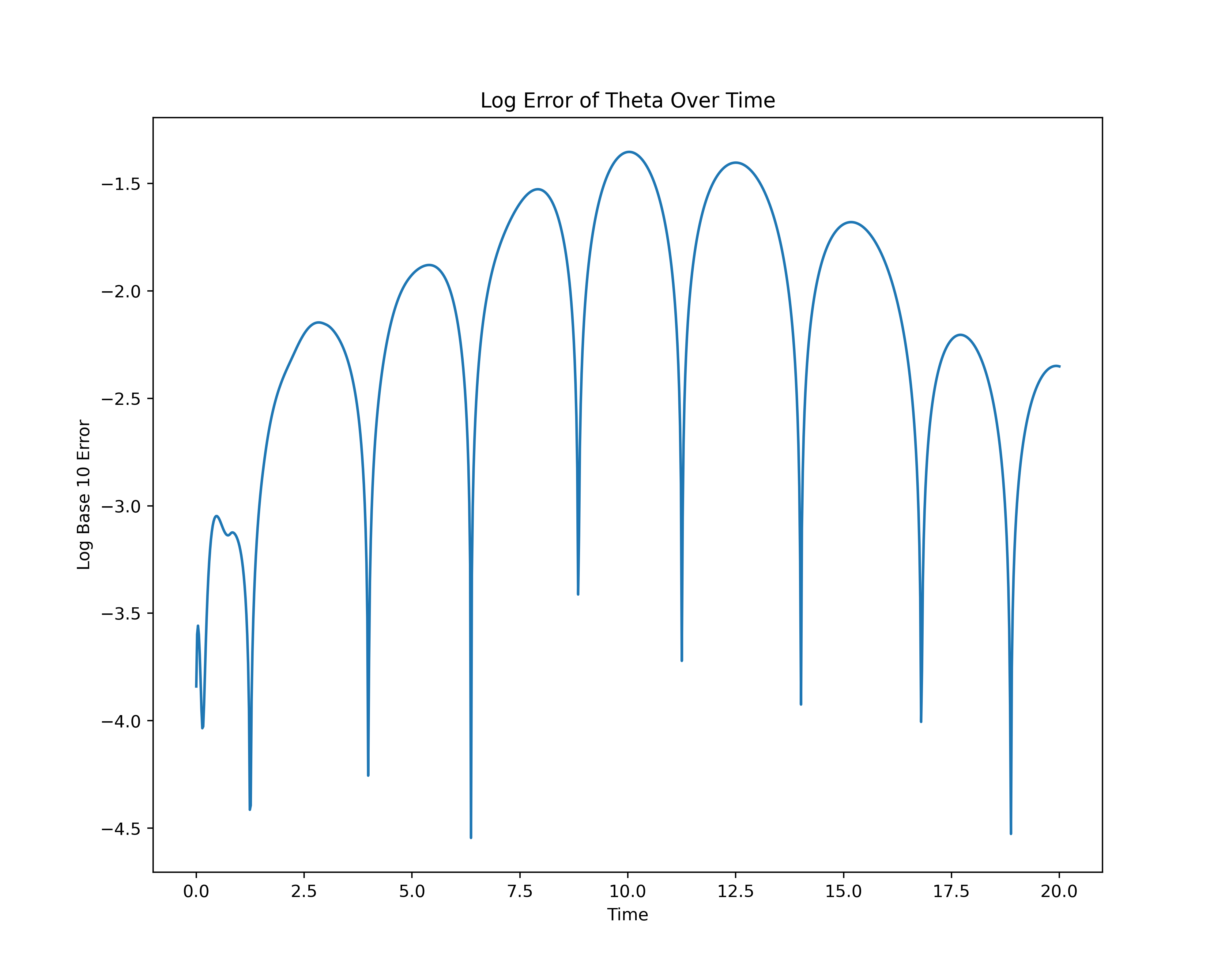
The log error plots above exhibit an interesting arching pattern
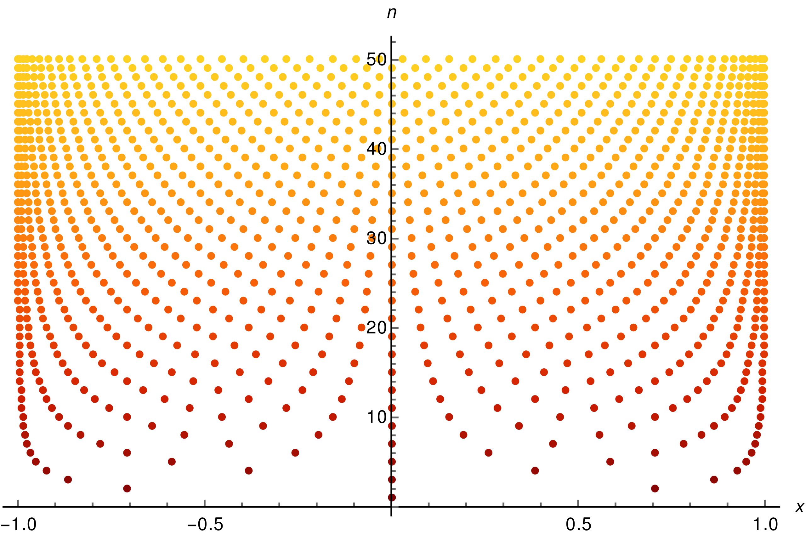
Finally, the observance of the Runge phenomenon suggests that Neural Networks can be thought of as interpolators instead of as approximators as the training loss approaches 0. Here is a link to the summary of a very interesting and thought provoking discussion between Prof. Yann LeCun and colleagues on Twitter from 2021.
Conclusion: Broader Implications and Future Research Directions
The pendulum problem, once a simple concept in classical mechanics, has evolved into a complex subject integral to contemporary engineering and science. Its journey began in the 17th century with Christiaan Huygens using it for timekeeping. This historical application laid the groundwork for further scientific breakthroughs, including Earth’s rotational proof and Galileo’s discoveries. In modern times, the pendulum transcends its initial purpose, playing a crucial role in seismology and structural engineering. Its principles, particularly in vibration control, are vital in designing earthquake-resistant structures. This evolution from a rudimentary timekeeping device to a key component in sophisticated systems highlights the pendulum’s significance. It exemplifies how basic mechanical concepts can be applied to solve complex, real-world problems. The story of the pendulum is a testament to the adaptability and enduring relevance of fundamental scientific principles.
Advancements in dynamical systems theory have led to a deeper understanding of the pendulum in realistic scenarios. Traditional models, previously simplistic, now incorporate external forces like air resistance and friction. These more complex models reveal intricate behaviors, including transitions to chaotic motions under certain conditions. This richer understanding has highlighted the limitations of conventional analytical methods, especially in predicting dynamic behaviors accurately. The need for advanced analytical approaches has become increasingly apparent. These approaches must capture the nuanced dynamics of systems like the pendulum. The challenge lies in accurately modeling systems that exhibit both regular and irregular behaviors. This advancement in understanding dynamical systems marks a significant evolution in scientific analysis and modeling.
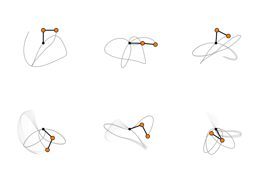
The emergence of numerical analysis has addressed the limitations of traditional methods in handling complex systems. In fields where precision and computational efficiency are paramount, such as aerospace engineering and high-rise building design, these methods are essential. The development of these techniques has been driven by the need for faster, more accurate solutions. These new methods aim to provide deeper insights into complex systems at reduced computational costs. The shift towards more efficient modeling techniques represents a significant change in computational analysis. It signals a new era in understanding and predicting the behavior of dynamic systems. The growing complexity of these systems necessitates a continual evolution of analytical methods. This evolution is crucial for keeping pace with the increasing sophistication of engineering and scientific applications.
The introduction of Neural Networks, especially the Physics-Informed Neural Network (PINN), has revolutionized the field. The Vanilla Neural Network (VNN) serves as a foundational model, leveraging function approximation capabilities. In contrast, the PINN introduces an innovative approach by integrating physics principles directly into the network. This allows the PINN to efficiently solve complex differential equations without extensive data reliance. These networks, particularly the PINN, have redefined predictive modeling in dynamics. They have opened new avenues for understanding and analyzing dynamic systems. The unique features of these networks demonstrate a significant advancement in the field. They highlight the potential for new, data-independent approaches to modeling dynamic systems with neural networks.

Looking forward, Operator Learning and methods like DeepONet represent the next frontier in dynamical system analysis. Building on the foundation laid by PINNs, these techniques hold great promise for solving complex differential equations.
Appendix
Image Credits: Thumbnail GIF by Chetvorno/Wikipedia
Project Code: Kal Parvanov/Github